Conditional formatting charts in excel
You can highlight elements and build a dynamic chart template. If you have Kutools for Excel installed you can apply its Select Same Different Cells feature to easily apply conditional formatting based on VLOOKUP and matching results in Excel.

Excel Magic Trick 626 Time Gantt Chart Conditional Formatting Data Validation Custom Formulas Gantt Chart Excel Gantt Chart Templates
But when she selects more than one worksheet in Excel now the conditional formatting option fades.
. Excel Conditional Formatting for Blank Cells. Conditional Formatting in Excel is used to highlight the data on the basis of some criteria. See tips below The selected cells now show Data Bars along with the original numbers.
We will show you how all this is possible. Enter the value 80 and select a formatting style. Excel Conditional Formatting.
Kutools for Excel- Includes more than 300 handy tools for ExcelFull feature free trial 60-day no credit card required. In our previous examples we have learned how to highlight based on the single-cell value. As you know Excel charts have some limits.
On the Excel Ribbon click the Home tab. On the Home tab in the Styles group click Conditional Formatting. In a nutshell conditional formatting charts can do way more things.
If the value is less than 2000 color the cell red. For each cell in the range B5B12 the first formula is evaluated. Say you want to create conditional formatting rules for the range B2.
Select Use a formula to determine which cells to format and enter the formula. Paula is wondering how she can apply conditional formatting to more than one sheet at a time. In this project you will learn how to analyze data and identify trends using a variety of tools in Microsoft Excel.
Conditional formatting allows you to automatically apply formattingsuch as colors icons and data barsto one or more cells based on the cell valueTo do this youll need to create a conditional formatting ruleFor example a conditional formatting rule might be. In this article we will learn how to color rows based on text criteria we use the Conditional Formatting option. We can apply the idea of conditional formatting to column charts by using multiple data series because the Excel feature applies only to cells not charts.
See the simple examples below. Conditional formatting rules are evaluated in order. Since the checkbox is linked to cell C2 this cell will have the value TRUE if the checkbox is checked and FALSE if its unchecked.
Click this link to see many more conditional formatting examples. B9 that will add a fill color to the cells when the checkbox is checked. We create short videos and clear examples of formulas functions pivot tables conditional formatting and charts.
We will apply conditional formatting so that the color of the circle changes as the progress changes. Excel changes the format of cell A1 automatically. Conditional formatting and charts are two tools that focus on highlighting and representing data in a visual form.
Note that the steps to apply pivot. From this we can highlight the duplicate color the cell as per different value ranges etc. 1Click Kutools Select Select Same Different.
Select the range you want to apply formatting to. And if youre familiar with the MATCH Function youll know that it returns the position of a value in a list and in this example that could be anything. On the Ribbon click the Home tab and then in the Styles group click Conditional Formatting.
Select a cell in the Excel table heading row. This chart displays a progress bar with the percentage of completion on a single metric. This technique just uses a doughnut chart and formulas.
In the list of conditional formatting options click Data Bars and then click one of the Data Bar options -- Gradient Fill or Solid Fill. The variance shown in column E is for reference only in this example and is not used by the conditional formatting rules. Custom shapes can improve this useful function.
See Conditional Formatting Rules. Change the value of cell A1 to 81. Use Excel conditional formatting to highlight worksheet cells automatically based on rules conditions that you set.
Make cells a different colour or change border font style or number format. Now if you remember my post from a couple of weeks ago with a similar example youll recall that I said Conditional Formatting formulas must always evaluate to TRUE or FALSE or their numeric equivalents of 1 and 0. Please do as follows.
This option is available in the Home Tab in the Styles group in Microsoft Excel. Excel highlights the cells that are greater than 80. This article will explain in detail the conditional formatting Conditional Formatting Conditional formatting is a technique in Excel that allows us to format cells in a worksheet based on certain conditions.
This works because Excel dates are serial numbers. Progress doughnut charts have become. In this resource well apply conditional formatting to a pivot table.
If you have Kutools for Excel installed you can use its Color Grouping Chart feature to quickly create a chart with conditional formatting in Excel. Formatting cells is easy in Excel. Conditional Formatting for Blank Cells is the function in excel that is used for creating inbuilt or customized formatting.
Here we have a table that shows monthly sales figures for a group of sales people. Rather it is conditional formatting applied to the table visually. The monthly sales quota is 5000 so lets use conditional formatting to highlight monthly sales numbers that are below that value.
Go to the worksheet named Example. Login details for this Free course will be emailed to you. Excel has a tool that automatically helps you out with that its called conditional formatting.
Click Highlight Cells Rules Greater Than. It is pretty easy to implement. IFB45TRUEFALSE Click the Format button and select your desired formatting.
With conditional formatting you can define rules to highlight cells using a range of color scales and icons and. Excel functions formula charts formatting creating excel dashboard others Please provide your correct email id. It seems that Microsoft did make this change as part of the ribbon-based user interface used in modern versions of Excel.
Rules can be based on a selected cells contents or values in a different cell. Conditional formatting is applied with rules. 1Select the data source you will create the chart based on and click Kutools Charts Color Grouping.
To see the existing Conditional Formatting Rules follow these steps. Example 2 Excel Conditional Formatting Based On Another Cell Value. In the Ribbon select Home Conditional Formatting New Rule.
Kutools for Excel- Includes more than 300 handy tools for ExcelFull feature free trial 30-day no credit card required. Conditional formatting is a very popular feature of Excel and is usually used to shade cells with different colors based on criteria that the user defines. How to Apply Conditional Formatting for Blank Cells.
Click OK then OK again to return to the Conditional Formatting Rules. In the Ribbon select Home Conditional Formatting Highlight Cells Rules Between You can either type in the bottom and top values or to make the formatting dynamic ie the result will change if you change the cells click on the cells that contain the bottom and top values. A common use case of conditional formatting is to highlight values in a set of data.
Take a closer look at the chart template. We create short videos and clear examples of formulas functions pivot tables conditional formatting and charts. Select the range you want to apply formatting to.
Besides background colors the Clear Conditional Formatting feature of Professor Excel Tools keeps all other common types of cell formatting font colors border etc. However if you treat column E as a helper column. Just select the cells you want to remove the rules from go to the Professor Excel ribbon and click on Clear Cond.
If youre ready to take your data organization game to the next level keep reading to learn how to use conditional formatting in Excel. Let us tell you that we have spent considerable time figuring this out. Youll use the value of cell C2 as the determinant for the.
It would be difficult to see various. Click Conditional Formatting then click Manage.

Info Graphics Rag Conditional Formatting In 3d Chart Youtube Chart Infographic Excel Dashboard Templates

Conditional Formatting Of Lines In An Excel Line Chart Using Vba Chart Excel Line Chart

Make Waffle Charts In Excel Using Conditional Formatting How To Pakaccountants Com Excel Microsoft Excel Tutorial Excel Hacks

Best Charts To Show Done Against Goal Excel Charts Excel Chart Excel Templates

Rag Conditional Formatting In Progress Circle Chart Progress Excel Rag

Conditional Formatting Rule Order For Task Checklist Microsoft Excel Tutorial Excel Excel Templates Project Management

Make Waffle Charts In Excel Using Conditional Formatting How To Pakaccountants Com Excel Excel Tutorials Excel Hacks
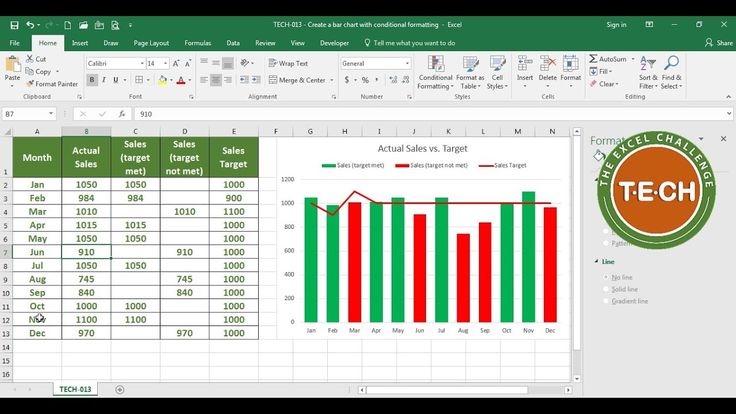
Tech 013 Create A Bar Chart With Conditional Formatting In Excel Youtube Excel Calendar Content Calendar Template Excel Calendar Template

Create Charts With Conditional Formatting

Moving X Axis Labels At The Bottom Of The Chart Below Negative Values In Excel Pakaccountants Com Excel Excel Tutorials Chart

Conditional Formatting In Multiple Batteries Graph In Excel Youtube Excel Graphing Goal Charts

Basic Conditional Formatting In Excel Access Using A Sales Example Exceldemy Excel Tutorials Excel Microsoft Excel

Conditional Formatting Intersect Area Of Line Charts Line Chart Chart Intersecting

Making A Slope Chart Or Bump Chart In Excel How To Pakaccountants Com Microsoft Excel Tutorial Excel Tutorials Excel

Excel Conditional Formatting In Depth Excel Tutorials Excel Text Symbols

Conditional Formatting Of Excel Charts Peltier Tech Blog Excel Spreadsheets Excel Bar Graphs

Excel Files With Temperature Charts And Conditional Formatting Bewitching Stitch Circulo Cromatico De Colores Colores Calidos Y Frios Clases De Arte